Can Artificial Dataset help to make up with lack of data in modern ML problems ?
In most of real life situations, gathering data intended to be used for training a learning algorithm just happen to be done either by hand or automatically.
This supposes that the developper of the model has access to the real-life situation where such data can be collected.
For instance, in the case of autonomous driving, imagery used for training can be recorded by a "simple" dashcam positioned at a precise spot. We put the experimenter in the condition of the prediction as he records data.

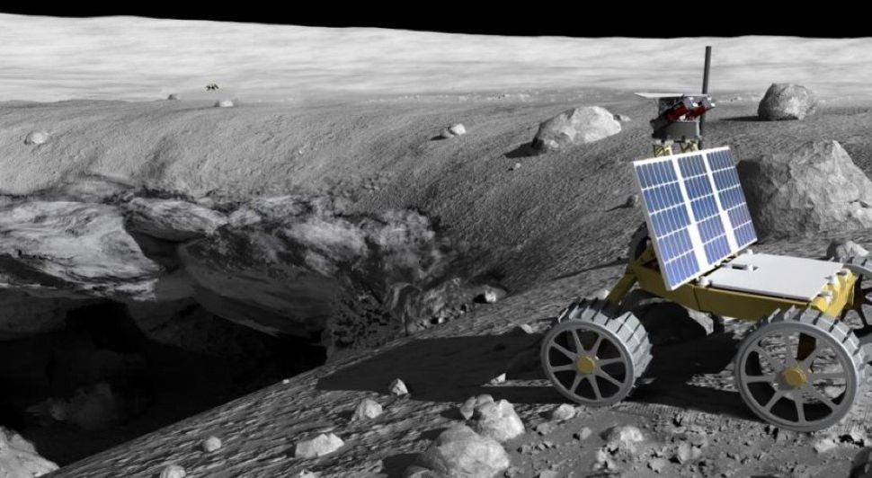
But there exists a lot of situation where Data is not easily, if not impossibly, collectable. One might think of pace Exploration and that is the subject of this analysis.
Machine Learning and more precisely Deep Learning have recently raised a lot of interest amongst the community of astrophysician for their ability to adapt to unknown situation: these properties of "generalisation" are what makes Deep Learning very efficient in such task. One example that we might think of is the use of Deep Learning for spacecraft docking. But what about Computer Vision ? As it is way cheaper to send a robot on the Moon than it is to send a Human, it may be very interesting to develop a highly efficient autonomous robot capable of moving and taking its own decisions, without having to wait for incoming messages that can take around 1.3 second to reach Earth's satellite and from 15 to 40 minutes to reach Mars (source: link).
However, the problem stays the same:
On which data could we train our model so that it performs as expected ?
The solution may lie right here, on Earth, and it is daily used by a lot of scientists: Simulation.
In this project, we will explore the role of simulation in Space Exploration, and more precisely, Computer Vision tasks related to Space Exploration by taking the example of rock semantic segmentation on the Moon.
Problem presentation: Semantic Segmentation of Rocks on a Moon-like landscapes
Imagine putting yourself in one of Nasa's scientist shoes (I know, it's a lot asking..) and you want to develop an an efficient way to have perform numerousous relevant analysis of the Moon surface. One good idea would be to send tons of small sized robot that would run around Moon's surface collecting data. However, they would be so many robots that it would be almost impossible to track all of them efficiently. It may then be reasonable to think about a way of making them autonomous. But how ? When Tesla wants to develop a Level 3 autonomous car, they just have to drive around and collect data while driving, it's "easy". But what our Moon explorers ?
How can they interpret their environment. One way to do so is through semantic segmentation:

Semantic segmentation is just attributing to each pixel of an image a class. In this example, extracted from our dataset, the 4 possible classes are:
- Small Rock (green)
- Big Rock (blue)
- Sky (red)
- Floor (black)
However, such imagery of real life high resolution pictures of the Moon surface are extremely rare. Hence, it cannot be considered a solution to just use them. This is where simulation comes into place. To illustrate it, let's dive in our dataset.
Our Dataset: Artificial Lunar Landscape Dataset (source: Kaggle)
This dataset, created and posted by Romain Pessia (whom I personally thank as it is a proof of very intense, time consuming but highly valuable work) consists of 9766 images of artificially created lunar landscape, of size 480x720 pixels, with semantically segmented rocks.

As well explained in the Dataset presentation, the images have been created using the following softwares:
"The software used for creating the images and their ground truth is Planetside Software's Terragen (https://planetside.co.uk/). The authors used NASA's LRO LOLA Elevation Model (https://astrogeology.usgs.gov/search/details/Moon/LRO/LOLA/Lunar_LRO_LOLA_Global_LDEM_118m_Mar2014/cub) as a source of large-scale terrain data."
So the main objective of this project will be to answer the following question:
Does training a network on artificial imagery helps when it comes to real-life situation ?
To evaluate this, we will:
- go through 4 different models of semantic segmentation so that we minimize the result bias linked to the model
- use real moon surface pictures with segmented rocks provided by Romain as well (a total of 36 images)
Our Models
When talking Semantic Segmentation, some very popular models come to mind (e.g. UNet-inspired models). This is the case here. Our 4 models will be:
- Basic UNet
- Feature Pyramidal Network
- LinkNet
- PSPNet
We will go through the implementation of each of these models by giving an overall explanation of their motivation and architecture. The goal of this project is neither to dive deep into Semantic Segmentation as a whole or to analyze the best possible model, it is to show how important artificially created Data could be some learning situation.
For my models, I used the Segmentation Models GitHub repository (link) where Models are hosted with already trained encoders (mostly VGG16).
UNet

Very popular when it comes to Semantic segmentation, the UNet model holds its name from the shape of its architecture (similar to a U). The first is, called the encoding phase, will shrink the size of the input image (or "downsample" it). The second phase will re-umsample it to set it back to its original size with, this time, every pixel segmented. This model has first been presented in this paper. To instantiate it and use it, I use the following Python code.
#Imports
import numpy as np
from keras.optimizers import Adam
import os
import tensorflow as tf
import matplotlib.pyplot as plt

#Third-party code
import segmentation_models as sm

#Personal code
from modules.utility_functions import get_size
from modules.data.dataManipulation import adjustData, predictionToMask, imageGenerator, testGenerator, saveResult
from modules.models.unet import jacard_coef_loss
#Constants
DATA_PATH = "../Data/images"

RELATIVE_TEST_FOLDER = "test/render"
RELATIVE_TEST_GT_FOLDER = "test/clean"
RELATIVE_RESULT_FOLDER = "test/results"

NUM_CLASSES = 4

IMAGE_SIZE=(256,256)

DATA_GEN_ARGS = dict(rotation_range=0.2,
                    width_shift_range=0.05,
                    height_shift_range=0.05,
                    shear_range=0.05,
                    zoom_range=0.05,
                    horizontal_flip=True,
                    fill_mode='nearest')
# Segmentation models losses can be combined together by '+' and scaled by integer or float factor
# set class weights for dice_loss (car: 1.; pedestrian: 2.; background: 0.5;)
dice_loss = sm.losses.DiceLoss(class_weights=np.array([0.5, 2, 1, 0.5]))
focal_loss = sm.losses.BinaryFocalLoss() if NUM_CLASSES == 1 else sm.losses.CategoricalFocalLoss()
total_loss = dice_loss + (1 * focal_loss)

# actulally total_loss can be imported directly from library, above example just show you how to manipulate with losses
# total_loss = sm.losses.binary_focal_dice_loss # or sm.losses.categorical_focal_dice_loss

metrics = [sm.metrics.IOUScore(threshold=0.5), sm.metrics.FScore(threshold=0.5)]
unet = sm.Unet('resnet34', classes=NUM_CLASSES, activation="softmax")
unet.load_weights("weights/12_10_2019_16_17_45/unet_moon_seg_17.hdf5")
unet.compile(optimizer = Adam(lr=7e-4, epsilon=1e-8, decay=1e-6), loss=total_loss, metrics=metrics)
Now that we have loaded our model, we will first test on artificially created data. The test on real Moon imagery will be after the review of all models and their performance.
with tf.device('/cpu:0'):

    testGen = imageGenerator(
        1,
        DATA_PATH,
        RELATIVE_TEST_FOLDER,
        RELATIVE_TEST_GT_FOLDER,
        DATA_GEN_ARGS,
        image_color_mode='rgb',
        mask_color_mode='rgb',
        num_class=NUM_CLASSES,
        target_size=IMAGE_SIZE,
        flag_multi_class = True)

    unet_test_metrics = unet.evaluate_generator(testGen, steps=500, verbose=1)
    print(unet_test_metrics, unet.metrics_names)
LinkNet

Based on this paper, the LinkNet models aimes to be a light-weights semantic segmentation model. It does not aim at the most accurate results but has a goal to provide real-time application. It mainly differs with the UNet architecture when it comes down to transmitting the encoder information back to the decoder. It no longer concatenates it but will instead add it.
When it comes down to code, the LinkNet behaviour and parameters are the same:
# Segmentation models losses can be combined together by '+' and scaled by integer or float factor
# set class weights for dice_loss (car: 1.; pedestrian: 2.; background: 0.5;)
dice_loss = sm.losses.DiceLoss(class_weights=np.array([0.5, 2, 1, 0.5]))
focal_loss = sm.losses.BinaryFocalLoss() if NUM_CLASSES == 1 else sm.losses.CategoricalFocalLoss()
total_loss = dice_loss + (1 * focal_loss)

# actulally total_loss can be imported directly from library, above example just show you how to manipulate with losses
# total_loss = sm.losses.binary_focal_dice_loss # or sm.losses.categorical_focal_dice_loss

metrics = [sm.metrics.IOUScore(threshold=0.5), sm.metrics.FScore(threshold=0.5)]
linknet = sm.Linknet(
    backbone_name="vgg16",
    input_shape=IMAGE_SIZE+(3,),
    classes=NUM_CLASSES, activation="softmax",
    encoder_weights='imagenet')

linknet.load_weights("weights/15_10_2019_08_12_52/linknet_moon_seg_19.hdf5")
linknet.compile(optimizer = Adam(lr=7e-4, epsilon=1e-8, decay=1e-6), loss=total_loss, metrics=metrics)
Now that we have loaded our model, we will first test on artificially created data. The test on real Moon imagery will be after the review of all models and their performance.
with tf.device('/cpu:0'):
    testGen = imageGenerator(
        1,
        DATA_PATH,
        RELATIVE_TEST_FOLDER,
        RELATIVE_TEST_GT_FOLDER,
        DATA_GEN_ARGS,
        image_color_mode='rgb',
        mask_color_mode='rgb',
        num_class=NUM_CLASSES,
        target_size=IMAGE_SIZE,
        flag_multi_class = True)

    linknet_test_metrics = linknet.evaluate_generator(testGen, steps=500, verbose=1)
    print(linknet_test_metrics, linknet.metrics_names)
PSPNet

The PSPNet (or Pyramid Scene Parsing Network) has first been introduced in this paper. It first uses a CNN to extract features that are then fed into a pyramid parsing module. This module is used to "harvest different sub-region representations" as explained in the paper. This step is then followed by an upsampling of each of these sub-regions to match the original feature map size. Then, this newly created representation (original feature maps + upsamples sub-region representations) are fed into a convolution layer that will get the per-pixel prediction, hence resulting in an efficient semantic segmentation process. By this pyramid scheme, this model is kind of "hard-coding" the concept of having different possible scales of the same object on a single image. This is the same intuition that was carried through the creation process of the FPN, that we will see right after.
PSP_IMAGE_SIZE = (288, 288) # has to be divisible by 48
# Segmentation models losses can be combined together by '+' and scaled by integer or float factor
# set class weights for dice_loss (car: 1.; pedestrian: 2.; background: 0.5;)
dice_loss = sm.losses.DiceLoss(class_weights=np.array([0.5, 2, 1, 0.5]))
focal_loss = sm.losses.BinaryFocalLoss() if NUM_CLASSES == 1 else sm.losses.CategoricalFocalLoss()
total_loss = dice_loss + (1 * focal_loss)

# actulally total_loss can be imported directly from library, above example just show you how to manipulate with losses
# total_loss = sm.losses.binary_focal_dice_loss # or sm.losses.categorical_focal_dice_loss

metrics = [sm.metrics.IOUScore(threshold=0.5), sm.metrics.FScore(threshold=0.5)]
psp = sm.PSPNet(backbone_name="vgg16", input_shape=PSP_IMAGE_SIZE+(3,), classes=NUM_CLASSES, activation="softmax", encoder_weights='imagenet')
psp.load_weights("weights/16_10_2019_13_23_33/psp_moon_seg_19.hdf5")
psp.compile(optimizer = Adam(lr=7e-4, epsilon=1e-8, decay=1e-6), loss=total_loss, metrics=metrics)
Now that we have loaded our model, we will first test on artificially created data. The test on real Moon imagery will be after the review of all models and their performance.
with tf.device('/cpu:0'):
    testGen = imageGenerator(
        1,
        DATA_PATH,
        RELATIVE_TEST_FOLDER,
        RELATIVE_TEST_GT_FOLDER,
        DATA_GEN_ARGS,
        image_color_mode='rgb',
        mask_color_mode='rgb',
        num_class=NUM_CLASSES,
        target_size=PSP_IMAGE_SIZE,
        flag_multi_class = True)

    psp_test_metrics = psp.evaluate_generator(testGen, steps=500, verbose=1)
    print(psp_test_metrics, psp.metrics_names)
FPN

The FPN (or Feature Pyramid Network) was detailed in this paper published just a few days after PSPNet. It uses the same concept of pyramid of scales but instead of concatenating them after having rescaled them, it will directly perform detection on each scaled feature map and will then concatenate the predictions. Therefore, each predictions are considered to be independent from each other, all providing their own context information. This very efficient network has been reused in numerous other projects such as the very famous Mask-RCNN.
# Segmentation models losses can be combined together by '+' and scaled by integer or float factor
# set class weights for dice_loss (car: 1.; pedestrian: 2.; background: 0.5;)
dice_loss = sm.losses.DiceLoss(class_weights=np.array([0.5, 2, 1, 0.5]))
focal_loss = sm.losses.BinaryFocalLoss() if NUM_CLASSES == 1 else sm.losses.CategoricalFocalLoss()
total_loss = dice_loss + (1 * focal_loss)

# actulally total_loss can be imported directly from library, above example just show you how to manipulate with losses
# total_loss = sm.losses.binary_focal_dice_loss # or sm.losses.categorical_focal_dice_loss

metrics = [sm.metrics.IOUScore(threshold=0.5), sm.metrics.FScore(threshold=0.5)]
fpn = sm.FPN(backbone_name="vgg16", input_shape=IMAGE_SIZE+(3,), classes=NUM_CLASSES, activation="softmax", encoder_weights='imagenet')
fpn.compile(optimizer = Adam(lr=7e-4, epsilon=1e-8, decay=1e-6), loss=total_loss, metrics=metrics)

fpn.load_weights("weights/13_10_2019_21_35_44/fpn_moon_seg_19.hdf5")
Now that we have loaded our model, we will first test on artificially created data. The test on real Moon imagery will be after the review of all models and their performance.
with tf.device('/cpu:0'):
    testGen = imageGenerator(
        1,
        DATA_PATH,
        RELATIVE_TEST_FOLDER,
        RELATIVE_TEST_GT_FOLDER,
        DATA_GEN_ARGS,
        image_color_mode='rgb',
        mask_color_mode='rgb',
        num_class=NUM_CLASSES,
        target_size=IMAGE_SIZE,
        flag_multi_class = True)

    fpn_test_metrics = fpn.evaluate_generator(testGen, steps=500, verbose=1)
    print(fpn_test_metrics, fpn.metrics_names)
fpn_test_metrics, unet_test_metrics, psp_test_metrics, linknet_test_metrics
Let's now try on real moon imagery where you would have sample such as these ones:


REAL_DATA_PATH = "../Data/real_moon_images"

REAL_RELATIVE_TEST_GT_FOLDER = "clean"
REAL_RELATIVE_RENDER_FOLDER = "shots"
with tf.device('/cpu:0'):

    testGen = imageGenerator(
        1,
        REAL_DATA_PATH,
        REAL_RELATIVE_RENDER_FOLDER,
        REAL_RELATIVE_TEST_GT_FOLDER,
        DATA_GEN_ARGS,
        image_color_mode='rgb',
        mask_color_mode='rgb',
        num_class=NUM_CLASSES,
        target_size=IMAGE_SIZE,
        flag_multi_class = True)

    unet_test_metrics = unet.evaluate_generator(testGen, steps=36, verbose=1)
    print(unet_test_metrics, unet.metrics_names)
with tf.device('/cpu:0'):
    testGen = imageGenerator(
        1,
        REAL_DATA_PATH,
        REAL_RELATIVE_RENDER_FOLDER,
        REAL_RELATIVE_TEST_GT_FOLDER,
        DATA_GEN_ARGS,
        image_color_mode='rgb',
        mask_color_mode='rgb',
        num_class=NUM_CLASSES,
        target_size=IMAGE_SIZE,
        flag_multi_class = True)

    linknet_test_metrics = linknet.evaluate_generator(testGen, steps=36, verbose=1)
    print(linknet_test_metrics, linknet.metrics_names)
with tf.device('/cpu:0'):
    testGen = imageGenerator(
        1,
        REAL_DATA_PATH,
        REAL_RELATIVE_RENDER_FOLDER,
        REAL_RELATIVE_TEST_GT_FOLDER,
        DATA_GEN_ARGS,
        image_color_mode='rgb',
        mask_color_mode='rgb',
        num_class=NUM_CLASSES,
        target_size=PSP_IMAGE_SIZE,
        flag_multi_class = True)

    psp_test_metrics = psp.evaluate_generator(testGen, steps=36, verbose=1)
    print(psp_test_metrics, psp.metrics_names)
with tf.device('/cpu:0'):
    testGen = imageGenerator(
        1,
        REAL_DATA_PATH,
        REAL_RELATIVE_RENDER_FOLDER,
        REAL_RELATIVE_TEST_GT_FOLDER,
        DATA_GEN_ARGS,
        image_color_mode='rgb',
        mask_color_mode='rgb',
        num_class=NUM_CLASSES,
        target_size=IMAGE_SIZE,
        flag_multi_class = True)

    fpn_test_metrics = fpn.evaluate_generator(testGen, steps=36, verbose=1)
    print(fpn_test_metrics, fpn.metrics_names)
As we can see, and as we could have expected, the performance on real moon images is under the performance on the samples from the training set but it still way more than usable:
fpn_test_metrics, unet_test_metrics, psp_test_metrics, linknet_test_metrics