# Currently the ‘memory growth’ option should be the same for all GPUs.
# You should set the ‘memory growth’ option before initializing GPUs.

import tensorflow as tf
gpus = tf.config.experimental.list_physical_devices('GPU')
if gpus:
    try:
        for gpu in gpus:
            tf.config.experimental.set_memory_growth(gpu, True)
    except RuntimeError as e:
        print(e)
TiSeLaC : Time Series Land Cover Classification Challenge
This challenge originating from this website challenges anyone who is interested to deal with SITS (Satellite Imagery Time Series).
The challenge involves a multi-class single label classification problem where the examples to classify are pixels described by the time series of satellite images and the prediction is related to the land cover of associated to each pixel:
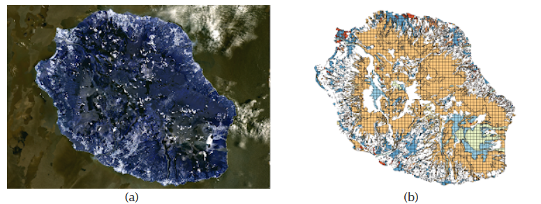
Before going in the EDA phase, we will first detail what our dataset is made of:

Data presentation
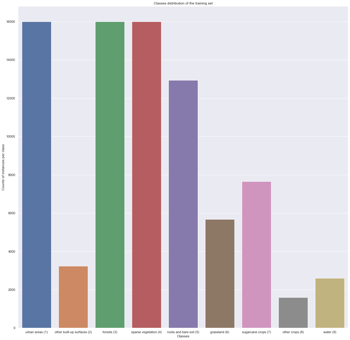
Training classes
The classes found in the training_class.txt file are the following:
| Class ID | Class Name | # Instances |
|---|---|---|
| 1 | Urban Areas | 16000 |
| 2 | Other built-up surfaces | 3236 |
| 3 | Forests | 16000 |
| 4 | Sparse Vegetation | 16000 |
| 5 | Rocks and bare soil | 12942 |
| 6 | Grassland | 5681 |
| 7 | Sugarcane crops | 7656 |
| 8 | Other crops | 1600 |
| 9 | Water | 2599 |
where the instances designates the pixels that makes up the image (total of 81714 pixels). It is important to note that not all pixel has a class, some are left blank.
Training file
The training file is in the form of a big text file where each row represents the value of the features of the given pixel at the 23 dates. As each pixel is described by 10 features (always in the following order: (Ultra Blue, Blue, Green, Red, NIR, SWIR1, SWIR2, NDVI, NDWI, BI), we have, for each row, 10*23 columns.
Coordinates file
This file gives the actual coordinates of pixels associated with a class to be able to draw a mask on the initial map of The Reunion Island.
Analysis of the source images
We will first explore the RGB component of the source images in the training file by redrawing its components.
# CONSTANTS & IMPORTS
import numpy as np
import pandas as pd
import time
import matplotlib.pyplot as plt
from tqdm import tqdm
import os
import cv2
import seaborn as sns;sns.set()

IMAGE_SIZE = (2866, 2633, 3)
NUM_OF_DAYS = 23
CLASSES = ["urban areas", "other built-up surfaces", "forests",
           "sparse vegetation", "rocks and bare soil", "grassland",
           "sugarcane crops", "other crops", "water"]
FEATURES = [
    "ultra blue","blue","green","red","NIR","SWIR1","SWIR2","NDVI","NDWI","BI"
]

NUM_OF_CLASSES = len(CLASSES)
NUM_OF_FEATURES = len(FEATURES)
NUM_OF_PIXELS = 81714
# DATA LOADING
data = pd.read_csv("data/train/training.txt", header=None)
coord = pd.read_csv("data/train/coord_training.txt", header=None)
classes_val = pd.read_csv("data/train/training_class.txt", header=None)

data_test = pd.read_csv("data/test/test.txt", header=None)
coord_test = pd.read_csv("data/test/coord_test.txt", header=None)
classes_val_test = pd.read_csv("data/test/test_class.txt", header=None)
y_test = classes_val_test.to_numpy()
img = [np.zeros(IMAGE_SIZE).astype(np.uint8) for _ in range(NUM_OF_DAYS)]
def row_to_img(row):

    idx = row.name

    coord_row = coord.iloc[idx, :]

    for i in range(23):
        b = row[i*10+1]
        g = row[i*10+2]
        r = row[i*10+3]

        #b = 255
        #g = 255
        #r = 255

        if (r > 255):
            r = 255
        if (b > 255):
            b = 255
        if (g > 255):
            g = 255

        img[i][coord_row[0], coord_row[1], :] = [r,g,b]

tqdm.pandas()
data.progress_apply(row_to_img, axis=1)
print("Images updated")
Checking the classes distribution
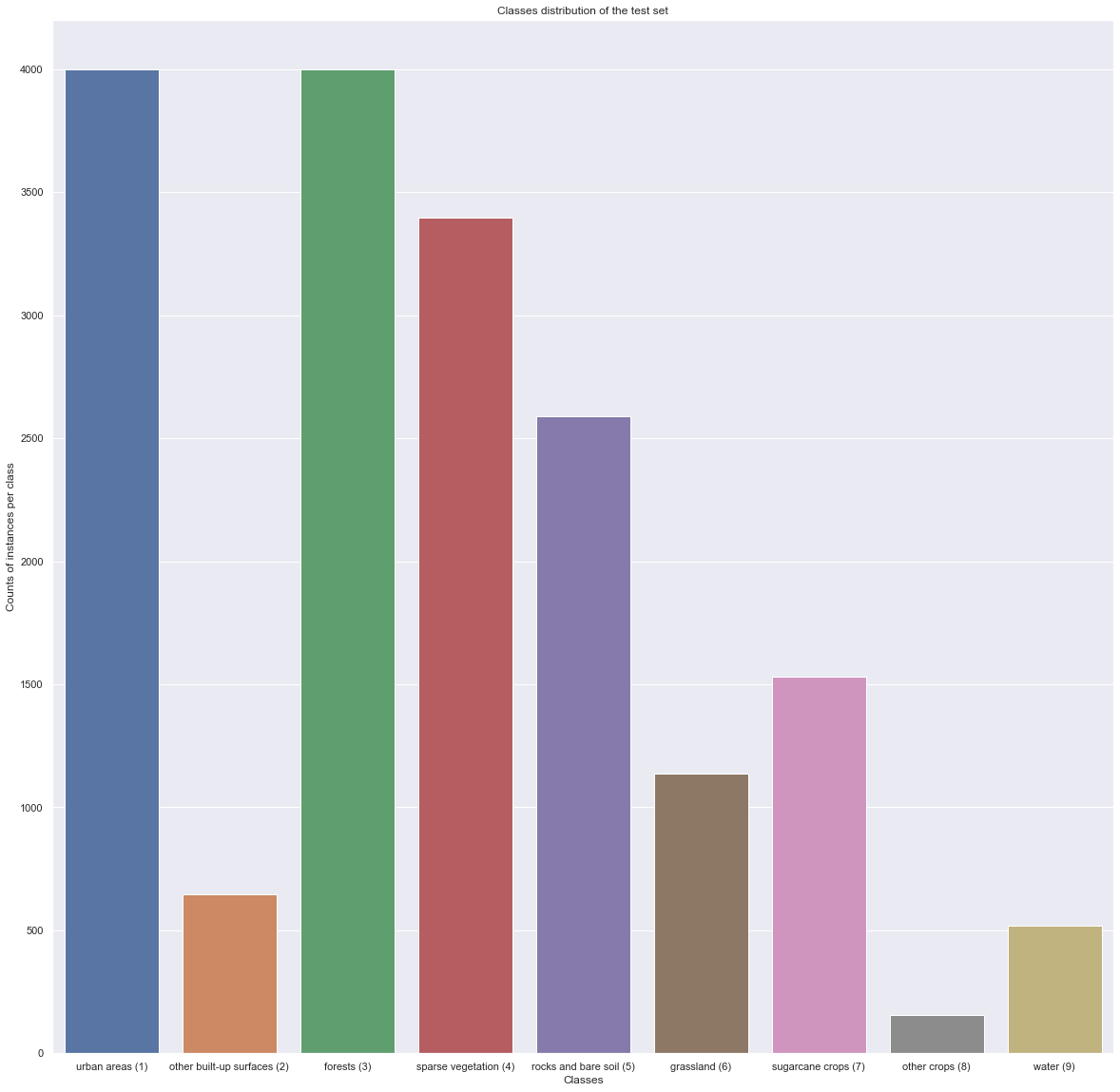
The subsampling of the pixels done by the TiSeLaC organizers had, as a first intent, the idea of balancing the classes distribution. We are then expecting to see a somewhat balanced dataset.
val_count = classes_val.iloc[:,0].value_counts().sort_index()
x, y = val_count.keys(), val_count.values
plt.figure(figsize = (20,20))
ax = sns.barplot([CLASSES[i] + f" ({i+1})" for i in range(len(CLASSES))], y)
ax.set_title("Classes distribution of the training set")
ax.set_ylabel("Counts of instances per class")
ax.set_xlabel("Classes")
plt.show()
val_count = classes_val_test.iloc[:,0].value_counts().sort_index()
x, y = val_count.keys(), val_count.values
plt.figure(figsize = (20,20))
ax = sns.barplot([CLASSES[i] + f" ({i+1})" for i in range(len(CLASSES))], y)
ax.set_title("Classes distribution of the test set")
ax.set_ylabel("Counts of instances per class")
ax.set_xlabel("Classes")
plt.show()
Plotting the 23 days images of the 81714 pixels
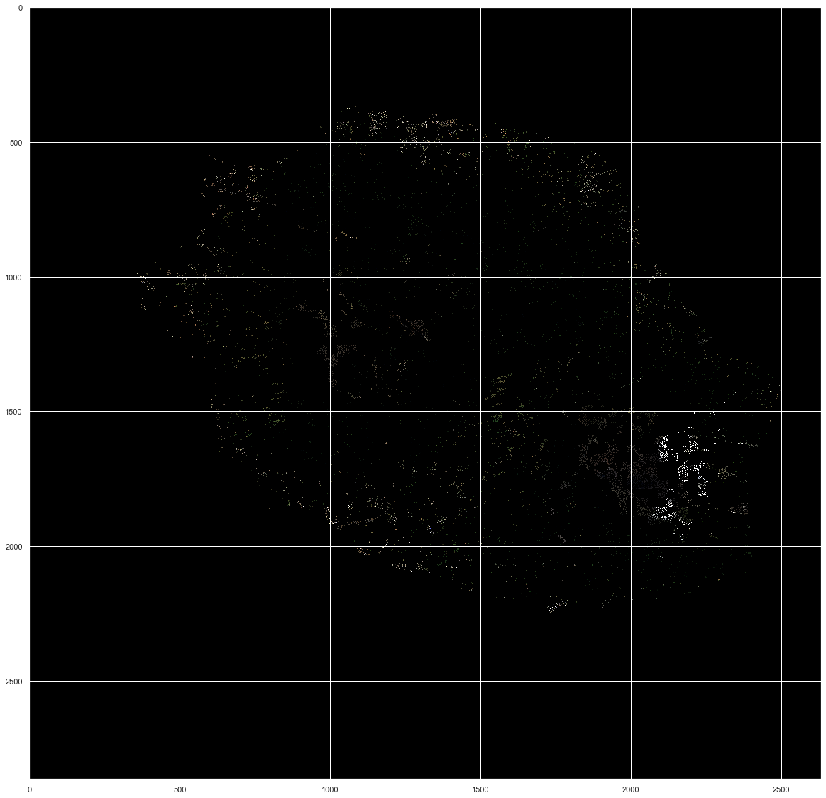
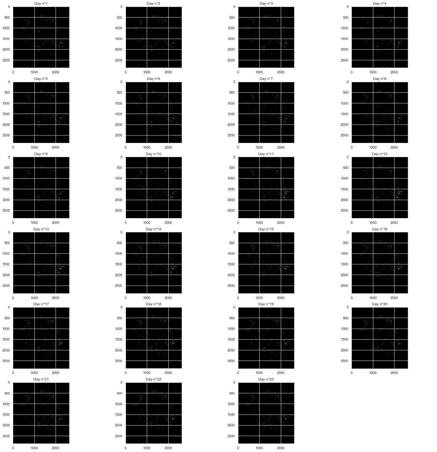
As out of the 2866*2633 pixels, only 81714 were retained, we cannot have a good overview of their position and variation in the images presented there. However, a few things are important to point out:
- We can notice clearly the shape of the Reunion island from the original image shown above
- Some changes in noticeable clusters of pixels can be observed, especially at the bottom right of the image
plt.figure(figsize = (20,20))
plt.imshow(img[13], aspect='auto')
# creating the gif
import imageio

# Write some Text

font                   = cv2.FONT_HERSHEY_SIMPLEX
bottomLeftCornerOfText = (1050,2600)
fontScale              = 5
fontColor              = (255,255,255)
lineType               = 4
thickness              = 10

scale_percent = 65 # percent of original size
width = int(img[0].shape[1] * scale_percent / 100)
height = int(img[0].shape[0] * scale_percent / 100)
dim = (width, height)
# resize image

with imageio.get_writer('day_animation.gif', mode='I') as writer:
    for i in range(0,NUM_OF_DAYS):
        for j in range(5):
            img_d = np.copy(img[i])
            cv2.putText(img_d,f'Day {i+1}',
                bottomLeftCornerOfText,
                font,
                fontScale,
                fontColor,
                thickness,
                lineType)
            resized = cv2.resize(img_d, dim, interpolation = cv2.INTER_NEAREST)
            writer.append_data(resized)
fig, axs=plt.subplots(6, 4, figsize=(20, 20), constrained_layout=True)

for i in range(0,NUM_OF_DAYS):

    x = int(i / 4)
    y = i % 4

    axs[x, y].imshow(img[i])

    axs[x,y].set_title(f'Day n°{i+1}')

fig.delaxes(axs[5,3])
#fig.tight_layout()
Giving insights on mean value of the 10 features over the 23 days, discriminated by class
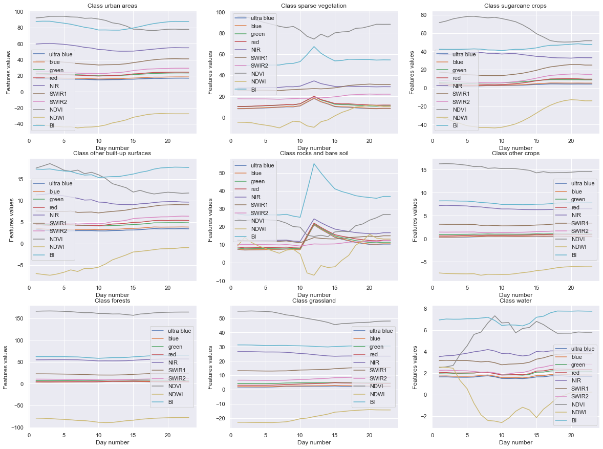
In order to see if we can extract any pattern ourselves, we will plot the mean value evolution of each feature over the 23 days by calculating the mean of these values for each class, resulting in one plot per class, with 10 lines on each plots.
# we start by building an array of 10 matrices of size 10*23 each

list_of_per_class_features_mean = [
    np.zeros((10,23)) for _ in range(len(CLASSES))
]

list_of_per_class_features_std = [
    np.zeros((10,23)) for _ in range(len(CLASSES))
]

N = data.shape[0]

def row_to_class(row):

    idx = row.name

    class_val = int(classes_val.iloc[idx, 0])

    # designates the feature
    for i in range(10):
        # designates the day
        for j in range(23):

            list_of_per_class_features_mean[class_val-1][i,j] += row[j*10 + i] # calculating the mean value

            list_of_per_class_features_std[class_val-1][i,j] += row[j*10 + i]*row[j*10 + i]/N

data.progress_apply(row_to_class, axis=1)
print("Calculation over..")
fig, axs = plt.subplots(3,3, figsize=(20,15))

for idx in range(len(list_of_per_class_features_mean)):

    i, j = idx % 3, int(idx / 3)

    values = list_of_per_class_features_mean[idx]/N

    standard_devs = list_of_per_class_features_std[idx] - np.square(values)

    for idx_f, feature in enumerate(FEATURES):

        x = np.arange(1,24)
        y = values[idx_f, :]

        e = np.sqrt(standard_devs[idx_f, :])

        axs[i, j].errorbar(x, y, label=feature)


    axs[i, j].set_title(f"Class {CLASSES[idx]}")
    axs[i, j].set_ylabel("Features values")
    axs[i, j].set_xlabel("Day number")
    axs[i, j].legend()
As we can see there, a few different classes see their features be highly disturbed through the days (e.g the water class or the rocks and bare soil are the most noticeable). Oppositely, the forests and crops classes are pretty steady in their results.
This apparent diversity in the variation of the features for each class is a good sign, it should not be too hard for an automatic classifier to be able to discriminate them from each other.
Classifiers
##  Keras imports
import tensorflow as tf
from tensorflow.keras.preprocessing import sequence
from tensorflow.keras.models import Sequential, Model
from tensorflow.keras.layers import Dense, Dropout, BatchNormalization, Input, Concatenate, Conv1D, MaxPooling1D
from tensorflow.keras.layers import LSTM, Flatten

from tensorflow.keras.optimizers import Adam, SGD
from tensorflow.keras.models import load_model
from tensorflow.keras.callbacks import ModelCheckpoint, EarlyStopping,ReduceLROnPlateau

## Sklearn imports
from sklearn.model_selection import train_test_split
from sklearn.preprocessing import OneHotEncoder, StandardScaler, MinMaxScaler

LR = 0.001
BATCH_SIZE = 256
EPOCHS = 50
VAL_SIZE = 0.1
1D-CNN
For this part, we will implement the Multi-Scale Convolutional Neural Networks presented in the following paper: Multi-Scale Convolutional Neural Networks for Time SeriesClassification
The architecture looks like this:

We will first setup our constants and imports
from tensorflow.keras.layers import Conv1D, Input, Concatenate, GlobalMaxPooling1D, MaxPooling1D
from tensorflow.keras.models import Model

LR = 0.01
BATCH_SIZE = 256
EPOCHS = 100
VAL_SIZE = 0.2
DOWN_SAMPLING_FACTOR = 2
DOWN_SAMPLING_SIZE = int(np.ceil(NUM_OF_DAYS)/DOWN_SAMPLING_FACTOR) + 1
SMOOTH_SIZE = 4

scaler = StandardScaler()
# Formatting the X data
data_train = data.to_numpy()
X = data_train.reshape((NUM_OF_PIXELS, 23, NUM_OF_FEATURES)).astype(np.int64)
coord_np = coord.to_numpy().astype(np.int32).reshape(-1, 2)
idx = np.arange(X.shape[0])

# Formatting the y data
classes_train = classes_val.to_numpy().astype(np.uint8)
enc = OneHotEncoder(handle_unknown='ignore', sparse=False)
y = enc.fit_transform(classes_train).astype(np.uint8)
# Splitting x and y into training and validation sets
X_train, X_val, y_train, y_val, idx_train, idx_val = train_test_split(X, y, idx, test_size = VAL_SIZE)
After splitting the image data, we take care of the pixel positions that we scale without data leak by fitting the transformer only to the training set.
coord_train = coord_np[idx_train]
coord_train = scaler.fit_transform(coord_train)

coord_val = scaler.transform(coord_np[idx_val])
Setting up the model
Here, we first create three simple models to extract features that may be specific to our three different scale of time series:
- The original time series
- The smoothed time series
- The down sampled time series
They are then concatenated and a new Convolutional layer is added before jumping to 3 fully connected layers. This model, in the same way than the LSTM, is pretty light in parameters, making its training relatively harder, hense requiring more advanced finetuning.
def get_base_model(input_len, fsize=6):
    #this base model represents the convolution + pooling phase (there will be three of it)

    input_seq = Input(shape=(input_len, 10))

    x = Conv1D(40, fsize, padding="same", activation="relu")(input_seq)
    x = MaxPooling1D()(x)
    model = Model(inputs=input_seq, outputs=x)

    return model

def get_coord_model():
    input_c = Input(shape=(2,))
    model = Model(inputs=input_c, outputs=input_c)

    return model

#it takes the original time series and its down-sampled versions as an input, and returns the result of classification as an output
def get_1D_CNN():

    input_original = Input(shape=(23, 10))
    input_multifrequency = Input(shape=(23 , 10))
    input_down_sampling = Input(shape=(DOWN_SAMPLING_SIZE, 10))

    base_net_original = get_base_model(23)
    base_net_multifrequency = get_base_model(23)
    base_net_down_sampling = get_base_model(DOWN_SAMPLING_SIZE, fsize=3)

    embedding_original = base_net_original(input_original)
    embedding_multifrequency = base_net_multifrequency(input_multifrequency)
    embedding_down_sampling = base_net_down_sampling(input_down_sampling)

    merged = Concatenate(axis=1)([embedding_original, embedding_multifrequency, embedding_down_sampling])#concatenate all the outputs

    conv = Conv1D(40, 6, padding="same", activation="relu")(merged)
    x = GlobalMaxPooling1D()(conv)

    coord_model = get_coord_model()
    #concatenating the coord model and the CNN-extracted features
    x = Concatenate(axis=-1)([x, coord_model.output])
    x = Dense(256, activation="relu")(x)
    x = Dense(128, activation="relu")(x)
    x = Dropout(0.3)(x)
    x = Dense(64, activation="relu")(x)
    #x = Dropout(0.3)(x)
    x = BatchNormalization()(x)
    x = Dense(32, activation="relu")(x)

    out = Dense(NUM_OF_CLASSES, activation='softmax')(x)

    model = Model(inputs=[input_original, input_multifrequency, input_down_sampling, coord_model.input], outputs=out)
    return model
Creating the data generator
We have to take care of the different scale of data by making sure that the generator, when taking one time series as an input, outputs three of them, one of which being the original, the two others having been through their own sets of processing.
def smoothing(row):
    # given a row of shape (23,10), smoothes all 10 feature according to the smoothing factor (mean over a SMOOTH_SIZE window)

    to_smooth = np.copy(row)

    for i in range(row.shape[1]):
        for j in range(row.shape[0]):

            smoothing_indices = np.array([k % row.shape[0] for k in range(int(j - SMOOTH_SIZE / 2), int(j + SMOOTH_SIZE / 2 + 1))])

            acc = 0
            for idx in smoothing_indices:
                acc += row[idx,i]

            to_smooth[j,i] = acc / SMOOTH_SIZE

    return to_smooth

def down_sampling(row):
    new_row = []

    for j in range(0, len(row)+1, DOWN_SAMPLING_FACTOR):
        new_row.append(row[j])

    return np.array(new_row)
def data_generator(X, y, input_shape=(23,10), batch_size=64):
    """
        X is a tuple (X_train, X_coord) where X_train is the pixels data and X_coord their coordinates
    """
    X_train, X_coord = X

    while True:

        for i in range(0, len(X_train), batch_size):

            upper = min(i+batch_size, len(X_train)-1)

            batch = np.copy(X_train[i:upper])
            smoothed = np.copy(X_train[i:upper])
            down_sampled = np.zeros((len(batch),DOWN_SAMPLING_SIZE,input_shape[1]))
            coords = np.copy(X_coord[i:upper])

            for row_idx in range(len(batch)):
                smoothed[row_idx, :] = smoothing(X_train[row_idx, :])
                down_sampled[row_idx, :] = down_sampling(X_train[row_idx, :])


            X_batch = [
                batch,smoothed,down_sampled, coords
            ]

            y_batch = y[i:upper]

            yield X_batch, y_batch
Training our model
train_gen = data_generator(
    (X_train,coord_train), y_train, batch_size=BATCH_SIZE)
val_gen = data_generator(
    (X_val,coord_val), y_val, batch_size=BATCH_SIZE)
train_steps = round(len(X_train) / BATCH_SIZE) + 1
val_steps = round(len(X_val) / BATCH_SIZE) + 1
model = get_1D_CNN()

opt = Adam(LR)
model.compile(opt, loss="categorical_crossentropy",
    metrics=['categorical_accuracy'])
model_filename = "tiselac-1d-cnn-{epoch:02d}-{val_loss:.2f}.h5"

callbacks = [
    ModelCheckpoint(
        os.path.join("models/", model_filename),
        monitor='val_loss', verbose=1, save_best_only=True, save_freq='epoch'),
    EarlyStopping(monitor='val_loss', min_delta = 1e-3, patience = 5),
    ReduceLROnPlateau(monitor='val_loss', factor=0.2, verbose=1,
                              patience=3, min_lr=0.00001)

]
model.fit_generator(
    train_gen,
    steps_per_epoch=train_steps,
    epochs=EPOCHS,
    validation_data=val_gen,
    validation_steps=val_steps,
    callbacks=callbacks
)
Testing the model
We will now test the model on the provided dataset and use a F1 Score metric for it (provided by Sk-Learn).
from sklearn.metrics import f1_score

data_test_np = data_test.to_numpy()

X_test = data_test_np.reshape((data_test_np.shape[0], 23, NUM_OF_FEATURES)).astype(np.float32)
coord_test_np = coord_test.to_numpy().astype(np.int32).reshape(-1, 2)
coord_test_np = scaler.transform(coord_test_np)

test_gen = data_generator((X_test,coord_test_np), y_test, batch_size=BATCH_SIZE)
test_steps = round(len(X_test) / BATCH_SIZE) + 1
y_pred = model.predict_generator(test_gen, steps=test_steps)
y_pred = np.argmax(y_pred, axis=1) +1
f1_score(y_test.flatten()[:17972], y_pred, average="weighted")
Advanced Classifiers
Based on this paper (Ismail Fawaz, H., Forestier, G., Weber, J. et al, 2019), I retained a number of the models compared.
1. Multi Channel Deep Convolutional Neural Network
Detailed in this paper (Zheng et al., 2014, 2016), this architecture want to exploit a presumed independence between the different features of the MTS data by applying convolution independently (in parallel) on each dimension of the input.
from tensorflow.keras.layers import Flatten, AveragePooling1D
def get_channel_model(ts_length):

    input_seq = Input(shape=(ts_length,1))

    x = Conv1D(12, 12, padding="same", activation="relu")(input_seq)
    x = MaxPooling1D()(x)
    x = Conv1D(24, 8, padding='same', activation="relu")(x)
    x = MaxPooling1D()(x)
    model = Model(inputs=input_seq, outputs=x)

    return model

def get_MCDCNN():

    input_models = [get_channel_model(23) for i in range(10)]

    merged = Concatenate(axis=1)([channel.input for channel in input_models])#concatenate all the outputs
    x = Flatten()(merged)
    x = Dense(732, activation="relu")(x)
    x = Dropout(0.3)(x)
    x = Dense(256, activation="relu")(x)
    x = BatchNormalization()(x)
    x = Dense(128, activation="relu")(x)
    x = Dense(NUM_OF_CLASSES, activation="softmax")(x)

    mcdcnn_model = Model([channel.input for channel in input_models], x)
    return mcdcnn_model
LR = 0.01
opt = SGD(LR, decay=0.0005)

mcdcnn_model = get_MCDCNN()
mcdcnn_model.compile(opt, loss="categorical_crossentropy",metrics=["accuracy"])
Starting training...
def data_generator_mcdcnn(X, y, input_shape=(10,23,1), batch_size=64):

    while True:

        for i in range(0, len(X), batch_size):

            upper = min(i+batch_size, len(X)-1)

            batch = np.copy(X[i:upper])

            batch = batch.reshape((batch.shape[0],)+input_shape)

            y_batch = y[i:upper]

            yield [batch[:,i,:,:] for i in range(10)], y_batch
model_filename = "tiselac-mcdcnn-{epoch:02d}-{val_loss:.2f}.h5"

callbacks = [
    ModelCheckpoint(
        os.path.join("models/", model_filename),
        monitor='val_loss', verbose=1, save_best_only=True, save_freq='epoch'),
    EarlyStopping(monitor='val_loss', min_delta = 1e-4, patience = 5),
    ReduceLROnPlateau(monitor='val_loss', factor=0.2, verbose=1,
                              patience=3, min_lr=0.00001)

]
X_train, X_val, y_train, y_val = train_test_split(X, y, test_size = VAL_SIZE)
BATCH_SIZE = 256
EPOCHS = 120

train_gen = data_generator_mcdcnn(X_train, y_train, batch_size=BATCH_SIZE)
val_gen = data_generator_mcdcnn(X_val, y_val, batch_size=BATCH_SIZE)
train_steps = round(len(X_train) / BATCH_SIZE) + 1
val_steps = round(len(X_val) / BATCH_SIZE) + 1

mcdcnn_model.fit_generator(
    train_gen,
    steps_per_epoch=train_steps,
    epochs=EPOCHS,
    validation_data=val_gen,
    validation_steps=val_steps,
    callbacks=callbacks
)
Testing the model
We will now test the model on the provided dataset and use a F1 Score metric for it (provided by Sk-Learn).
from sklearn.metrics import f1_score

data_test_np = data_test.to_numpy()

X_test = data_test_np.reshape((data_test_np.shape[0], 23, NUM_OF_FEATURES)).astype(np.float32)

test_gen = data_generator_mcdcnn(X_test, y_test, batch_size=BATCH_SIZE)
test_steps = round(len(X_test) / BATCH_SIZE) + 1
y_pred = mcdcnn_model.predict_generator(test_gen, steps=test_steps)
y_pred = np.argmax(y_pred, axis=1) +1
test_gen = data_generator_mcdcnn(X_test, y_test, batch_size=BATCH_SIZE)
f1_score(y_test.flatten()[:-1], y_pred[:17972], average="weighted")
2. Time-CNN
Seen as an improvement of the MCDCNN method, by training multivariate time series jointly for better feature extraction, this architecture has been developed in this paper (Zhao B, Lu H, Chen S, Liu J, Wu D , 2017).
Multiple unique characteristics are notable:
- A MSE loss used with a sigmoid output layer
- Use of Average pooling instead of Max Pooling
- No Pooling layer after the last convolution layer before the feature extracted classification
def get_time_cnn(input_shape=(23,10)):

    input_l = Input(input_shape)
    x = Conv1D(24, 8, activation="relu")(input_l)
    x = AveragePooling1D(pool_size=3)(x)
    x = Conv1D(24, 4, activation="relu")(x)
    x = Flatten()(x)
    x = Dense(128, activation="relu")(x)
    x = Dropout(0.3)(x)
    x = Dense(64, activation="relu")(x)
    x = BatchNormalization()(x)
    x = Dense(32, activation="relu")(x)
    x = Dense(NUM_OF_CLASSES, activation='sigmoid')(x)

    model = Model(input_l, x)
    return model
LR = 0.001
opt = Adam(LR, decay=0)

time_cnn = get_time_cnn()
time_cnn.compile(opt, loss="mse")
model_filename = "tiselac-time-cnn-{epoch:02d}-{val_loss:.2f}.h5"

callbacks = [
    ModelCheckpoint(
        os.path.join("models/", model_filename),
        monitor='val_loss', verbose=1, save_best_only=True, save_freq='epoch'),
    EarlyStopping(monitor='val_loss', min_delta = 1e-4, patience = 5),
    ReduceLROnPlateau(monitor='val_loss', factor=0.2, verbose=1,
                              patience=3, min_lr=0.00001)

]
BATCH_SIZE = 128
EPOCHS = 2000

time_cnn.fit(
    X_train, y_train,
    epochs=EPOCHS,
    batch_size=BATCH_SIZE,
    validation_data=(X_val, y_val),
    callbacks=callbacks
)
Testing the model
We will now test the model on the provided dataset and use a F1 Score metric for it (provided by Sk-Learn).
from sklearn.metrics import f1_score

data_test_np = data_test.to_numpy()

X_test = data_test_np.reshape((data_test_np.shape[0], 23, NUM_OF_FEATURES)).astype(np.float32)
y_pred = time_cnn.predict(X_test)
y_pred = np.argmax(y_pred, axis=1) +1
f1_score(y_test.flatten(), y_pred, average="weighted")
Merge of Multimodal/Unimodal architecture
We will first work with Deep Learning oriented solution and try implementing an LSTM on this data. Let's setup our working environment with the adequate hyperparameters.
LR = 0.001
BATCH_SIZE = 256
EPOCHS = 50
VAL_SIZE = 0.1
Setting up the data (splitting into training and validation sets)
scaler_coord = StandardScaler()

# Formatting the X data
data_train = data.to_numpy()
#data_train = minmax_scaler.fit_transform(data_train)

data_coord = coord.to_numpy().astype(np.int32).reshape(-1, 2)
data_coord = scaler_coord.fit_transform(data_coord)


X = data_train.reshape((NUM_OF_PIXELS, 23, NUM_OF_FEATURES)).astype(np.int32)


# Formatting the y data
classes_train = classes_val.to_numpy().astype(np.uint8)
enc = OneHotEncoder(handle_unknown='ignore', sparse=False)
y = enc.fit_transform(classes_train).astype(np.uint8)
# Splitting x and y into training and validation sets
indices = np.arange(X.shape[0])
X_train, X_val, y_train, y_val, idx_train, idx_val = train_test_split(X, y, indices, test_size = VAL_SIZE)
X_train_formatted = [
    X_train,
    #X_train
    data_coord[idx_train]
]
X_train_formatted.extend([np.expand_dims(X_train[:,:,i], axis=2) for i in range(10)])

X_val_formatted = [
    X_val,
    #X_val
    data_coord[idx_val]
]
X_val_formatted.extend([np.expand_dims(X_val[:,:,i], axis=2) for i in range(10)])
Setting up the model
model_filename = "tiselac-time-cnn-{epoch:02d}-{val_loss:.2f}.h5"

callbacks = [
    ModelCheckpoint(
        os.path.join("models/", model_filename),
        monitor='val_loss', verbose=1, save_best_only=True, save_freq='epoch'),
    #EarlyStopping(monitor='val_loss', min_delta = 1e-3, patience = 6),
    ReduceLROnPlateau(monitor='val_loss', factor=0.2, verbose=1,
                              patience=3, min_lr=0.00001)


]
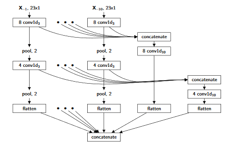
def get_multivariate_model():
    """
        Treats the data of each band as a multimodal time serie
    """
    input_lstm = Input((23, 10))
    #lstm = LSTM(512, input_shape=(23, 10))(input_lstm)

    conv = Conv1D(32, 3, padding="same", activation="relu")(input_lstm)
    conv = Conv1D(32, 3, padding="same", activation="relu")(conv)
    conv = Conv1D(32, 3, padding="same", activation="relu")(conv)
    flat = Flatten()(conv)

    return Model(inputs=input_lstm,outputs=flat)

def get_coordinates_model():
    """
        Treats the pixel coordinates on the image
    """
    input_seq = Input(shape=(2,))

    #x = Conv1D(32, 3, padding="same", activation="relu")(input_seq)
    #x = MaxPooling1D()(x)
    #x = Conv1D(32, 3, padding="same", activation="relu")(x)

    return Model(inputs=input_seq, outputs=input_seq)

def get_univariate_models():
    """
        Treats each band independently then concatenate models in one single
    """
    # Models built for each band
    inputs = [Input((23,1)) for _ in range(10)]
    convs1 = [Conv1D(8,3,padding="same",activation="relu")(inputs[i]) for i in range(10)]
    pools = [MaxPooling1D()(convs1[i]) for i in range(10)]
    convs2 = [Conv1D(4,3,padding="same",activation="relu")(pools[i]) for i in range(10)]
    pools = [MaxPooling1D()(convs2[i]) for i in range(10)]
    flatt = [Flatten()(pools[i]) for i in range(10)]


    # First concatenate: each band at the first convolutional level
    conca1 = Concatenate()(convs1)
    conv1 = Conv1D(8,10,padding="same",activation="relu")(conca1)
    flatt1 = Flatten()(conv1)
    flatt.append(flatt1)

    # Second concatenate: each band at the second convolutional level
    conca2 = Concatenate()(convs2)
    conv2 = Conv1D(4,10,padding="same",activation="relu")(conca2)
    flatt2 = Flatten()(conv2)
    flatt.append(flatt2)

    # Third and last concatenate after every flatten, adding the process of the first and second concats
    conca3 = Concatenate()(flatt)

    return Model(inputs=inputs, outputs=conca3)

# Merging inputs from the time series and the pixel position
mult_model = get_multivariate_model()
coord_model = get_coordinates_model()
univ_models = get_univariate_models()


merged = Concatenate(axis=-1)([
    mult_model.output,
    coord_model.output,
    univ_models.output])

x = Dense(256, activation="relu")(merged)
x = Dense(128, activation="relu")(x)
x = Dropout(0.3)(x)
x = Dense(64, activation="relu")(x)
x = Dropout(0.3)(x)
x = Dense(32, activation="relu")(x)
out = Dense(NUM_OF_CLASSES, activation='softmax')(x)

model = Model(inputs=[
    mult_model.input,
    coord_model.input,
    univ_models.input], outputs=[out])

opt = Adam(LR)

model.compile(opt, loss="categorical_crossentropy",
    metrics=['categorical_accuracy'])
model.fit(
    X_train_formatted, y_train, batch_size=BATCH_SIZE, epochs=EPOCHS, verbose=1,
    callbacks=callbacks,
    validation_data=(X_val_formatted, y_val))
Testing the model
We will now test the model on the provided dataset and use a F1 Score metric for it (provided by Sk-Learn).
from sklearn.metrics import f1_score, confusion_matrix

data_test_np = data_test.to_numpy()
#data_test_np = data_test_np.transform(minmax_scaler)

X_test = data_test_np.reshape((data_test_np.shape[0], 23, NUM_OF_FEATURES)).astype(np.float32)
coord_test_np = coord_test.to_numpy().astype(np.int32).reshape(-1, 2)
coord_test_np = scaler_coord.transform(coord_test_np)

univariate_bands = [np.expand_dims(X_test[:,:,i], axis=2) for i in range(10)]

X_test = [
    X_test,
    #X_test
    coord_test_np
]
X_test.extend(univariate_bands)

y_pred = model.predict(X_test)
y_pred = np.argmax(y_pred, axis=1) +1
We evaluate the F1 score to compare with other teams result in the context of the TiSeLaC challenge.
f1_score(y_test.flatten(), y_pred, average="weighted")
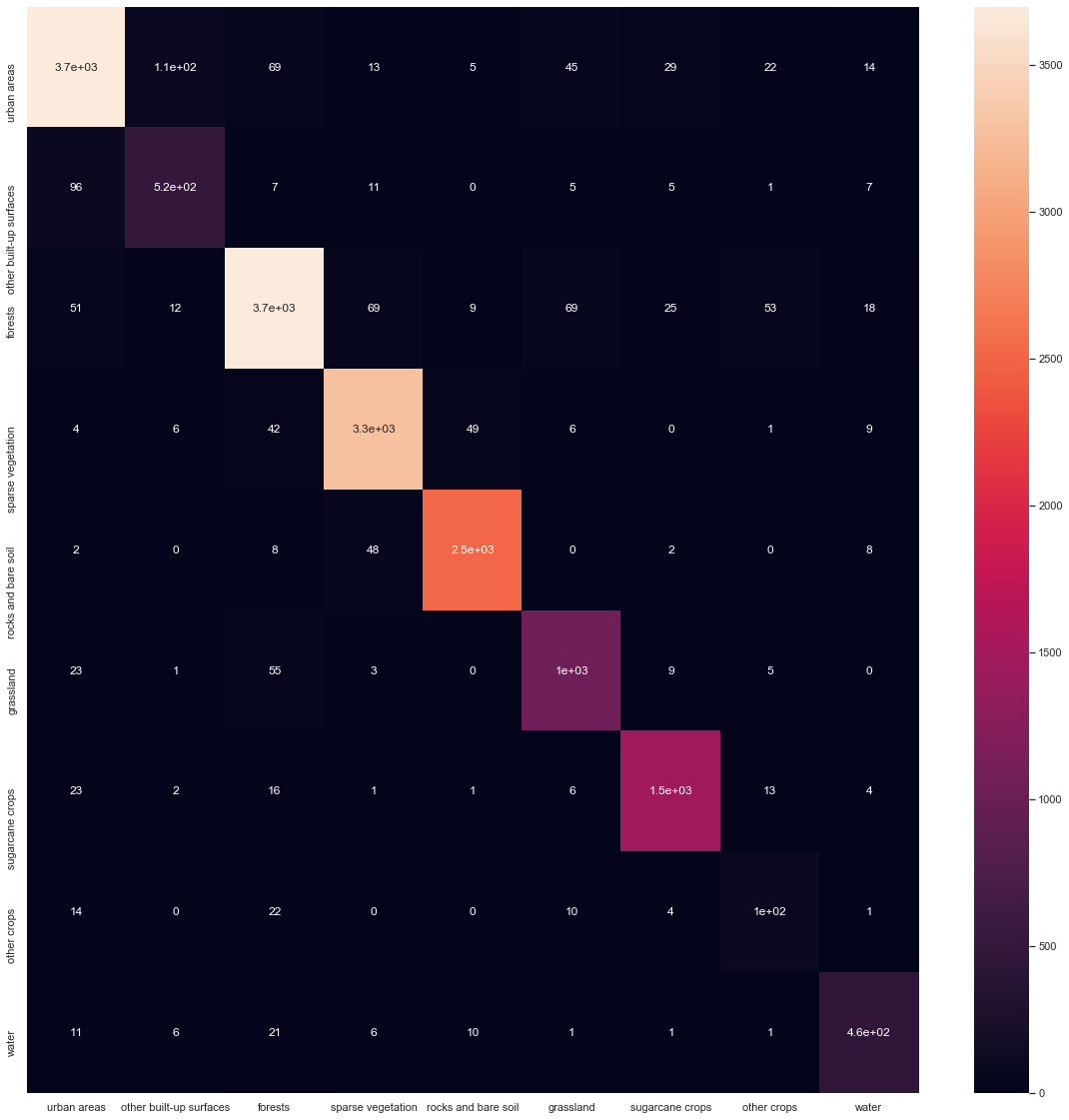
To have better insights on which classes are often misclassified, we will plot a confusion matrix using seaborn and sklearn.
m = confusion_matrix(y_test.flatten(), y_pred)
m_pd = pd.DataFrame(m)
classes_as_dict = {i: CLASSES[i] for i in range(9)}
m_pd = m_pd.rename(columns=classes_as_dict, index=classes_as_dict)
figs, axs = plt.subplots(figsize=(20,20))
sns.heatmap(m_pd, ax=axs, annot=True)
